Within the dynamic field of Human Resources (HR), where employees are an organization’s lifeblood, data-driven decision-making has emerged as a critical component of successful strategic planning. HR experts might use Minitab, a powerful statistical program, as a guide while managing the large amount of data. This article explores the complexities of Minitab, examining parametric and non-parametric tests, illuminating how they are used in HR contexts, and offering comprehensive explanations accompanied by practical examples.
Parametric tests and non-parametric tests are two broad categories of statistical tests used to analyze data in research and draw conclusions. The distinction between them lies in the assumptions they make about the underlying distribution of the data.
Parametric Tests:
Parametric tests are statistical tests that assume the data being analyzed follows a specific distribution, most commonly the normal distribution. These tests are characterized by their reliance on parameters (such as means and variances) of the assumed distribution. Key characteristics of parametric tests include:
- Assumption of Normality: Parametric tests assume that the data is normally distributed. This means that the values of the variable being measured follow a bell-shaped curve.
- Known Population Parameters: Parametric tests often require knowledge of population parameters, such as the population mean and standard deviation. In practice, these parameters are estimated from sample data.
- Scale of Measurement: Parametric tests are often suitable for continuous and interval data, where the intervals between values are meaningful.
- Greater Statistical Power: Parametric tests are generally more powerful (i.e., more likely to detect a true effect) when their assumptions are met.
Common parametric tests include t-tests, analysis of variance (ANOVA), regression analysis, and parametric correlation coefficients (e.g., Pearson correlation).
Non-Parametric Tests:
Non-parametric tests, on the other hand, make fewer assumptions about the underlying distribution of the data. These tests are often used when the data does not meet the normal distribution assumptions or when dealing with ordinal or categorical data. Key characteristics of non-parametric tests include:
- Distribution-Free: Non-parametric tests are distribution-free or less dependent on the shape of the distribution. They do not assume a specific distribution for the data.
- Less Stringent Assumptions: Non-parametric tests are more robust and suitable for data that may not meet the strict assumptions of normality or homogeneity of variances.
- Ordinal or Nominal Data: Non-parametric tests are often used for ordinal or nominal data, where the order or categories have meaning but the intervals between values may not.
- Less Statistical Power: Non-parametric tests are generally less powerful than their parametric counterparts. They may require larger sample sizes to achieve similar levels of statistical significance.
Common non-parametric tests include the Mann-Whitney U test, Wilcoxon signed-rank test, Kruskal-Wallis test, and Chi-square test.
When to Use Which:
The choice between parametric and non-parametric tests depends on the nature of the data and whether the assumptions of parametric tests are met. If the data is approximately normally distributed and meets other parametric assumptions, parametric tests are often preferred due to their greater statistical power. However, if the assumptions are violated or the data is not conducive to parametric testing, non-parametric tests provide a robust alternative for drawing meaningful conclusions.
What is normal data?
Normal data, also known as normally distributed data, follows a specific statistical distribution known as the normal distribution or Gaussian distribution. The normal distribution is a symmetric, bell-shaped probability distribution that is characterized by its mean (average) and standard deviation. In a normal distribution:
- Symmetry: The distribution is symmetric around its mean, which is located at the center of the distribution.
- Bell-shaped Curve: The majority of the data falls close to the mean, with fewer values as you move away from the center in either direction.
- 68-95-99.7 Rule: Approximately 68% of the data falls within one standard deviation of the mean, 95% within two standard deviations, and 99.7% within three standard deviations.
- Parameters: The distribution is completely defined by its mean and standard deviation.
Mathematically, the probability density function (PDF) of a normal distribution is given by the formula:
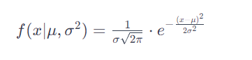
where:
- μ is the mean,
- σ is the standard deviation,
- x is a specific data point,
- e is the base of the natural logarithm.
Normal distributions are widely used in statistics due to the central limit theorem, which states that the distribution of the sum (or average) of a large number of independent, identically distributed random variables approaches a normal distribution, regardless of the original distribution.
In practical terms, if a dataset is approximately normally distributed, it implies that most values cluster around the mean, making it easier to make statistical inferences and predictions. Normality assumptions are crucial for certain parametric statistical tests, such as t-tests and analysis of variance (ANOVA). Researchers often check for normality using statistical tests (e.g., Shapiro-Wilk test) or graphical methods (e.g., histograms or Q-Q plots) before applying these tests.
Methods of checking Normality:
There are several methods to check the normality of data, ranging from graphical methods to statistical tests. Keep in mind that no single method is foolproof, and it’s often advisable to use a combination of approaches for a more comprehensive assessment. Here are common ways to check for normality:
Graphical Methods:
- Histogram:
- Plot a histogram of the data and visually assess if it resembles a bell-shaped curve.
- Q-Q (Quantile-Quantile) Plot:
- A Q-Q plot compares the quantiles of the sample data against the quantiles of a theoretical normal distribution. If the points fall along a straight line, it indicates normality.
- Box Plot:
- Box plots can give a sense of the symmetry and spread of the data. Normally distributed data tends to have a symmetrical box plot.
- P-P (Probability-Probability) Plot:
- Similar to Q-Q plots, P-P plots compare the cumulative distribution function of the sample data to that of a theoretical normal distribution.
Statistical Tests:
Shapiro-Wilk Test:
- The Shapiro-Wilk test is a widely used statistical test for normality. The null hypothesis is that the data follows a normal distribution. A low p-value (< 0.05) indicates departure from normality.
- To perform the Shapiro-Wilk test in Minitab, follow these steps:
- Input your data into a column in Minitab.
- Go to “Stat” > “Basic Statistics” > “Normality Test.”
- In the dialog box, select the column containing your data.
- Choose the Shapiro-Wilk test.
- Click “OK.”
- Minitab will provide output, including the test statistic and p-value. A low p-value (< 0.05) suggests departure from normality.
Anderson-Darling Test:
Similar to the Shapiro-Wilk test but often more sensitive, especially for larger sample sizes.
To conduct the Anderson-Darling test in Minitab:
- Input your data into a column.
- Go to “Stat” > “Basic Statistics” > “Normality Test.”
- Select the column with your data.
- Choose the Anderson-Darling test.
- Click “OK.”
Minitab will produce output, including the Anderson-Darling statistic and critical values. Larger values of the statistic indicate a greater departure from normality.
Kolmogorov-Smirnov Test:
- This test compares the sample distribution to a theoretical normal distribution. The null hypothesis is that the data follows a normal distribution.
For the Kolmogorov-Smirnov test in Minitab:
- Input your data into a column.
- Go to “Stat” > “Basic Statistics” > “Normality Test.”
- Select the column with your data.
- Choose the Kolmogorov-Smirnov test.
- Click “OK.”
Minitab will provide output, including the test statistic and p-value. A low p-value suggests deviation from normality.
Numerical Summaries:
Skewness and Kurtosis:
- Skewness measures the asymmetry of the distribution, and kurtosis measures the “tailedness” of the distribution. Normal distributions have skewness around 0 and kurtosis around 3.
Shapiro-Francia Test:
- Similar to the Shapiro-Wilk test, but may be less sensitive to extreme values.
Skewness and Kurtosis:
To compute skewness and kurtosis in Minitab:
- Input your data into a column.
- Go to “Stat” > “Basic Statistics” > “Display Descriptive Statistics.”
- Choose the column containing your data.
- Check the options for skewness and kurtosis.
- Click “OK.”
Minitab will display output with skewness and kurtosis values.
Classification of Data:
In statistics, data can be classified into various types based on its nature, characteristics, and level of measurement. Understanding the different types of data is crucial for choosing appropriate statistical analyses and drawing meaningful conclusions. Here are the primary types of data:
1. Nominal Data:
- Nominal data represents categories or labels without any inherent order or ranking. Each category is distinct and unrelated. Examples include gender (male/female), colors (red, blue, green), or types of fruits (apple, orange, banana). Nominal data can be coded or assigned numbers for analysis, but these numbers don’t imply any inherent order.
2. Ordinal Data:
- Ordinal data consists of categories with a meaningful order or ranking, but the intervals between them are not uniform or meaningful. The differences between categories are not well-defined. Examples include education levels (high school, bachelor’s, master’s), customer satisfaction ratings (poor, fair, good, excellent), or socioeconomic classes (lower, middle, upper). While you can determine the order, you cannot quantify the differences between the categories.
3. Interval Data:
- Interval data has a meaningful order between categories, and the intervals between values are equal and meaningful. However, it lacks a true zero point, meaning zero does not indicate the absence of the quantity being measured. Examples include temperature measured in Celsius or Fahrenheit, IQ scores, or calendar years. In interval data, addition and subtraction operations are meaningful, but multiplication and division are not.
4. Ratio Data:
- Ratio data has a meaningful order, equal intervals between values, and a true zero point, indicating the absence of the quantity being measured. Ratio data allows for meaningful mathematical operations, including multiplication and division. Examples include height, weight, age, income, and distance. Ratio data provides the most information and flexibility for statistical analysis.
5. Categorical Data:
- Categorical data is a broad term encompassing both nominal and ordinal data. It represents groups or categories and can be used to label variables. Categorical data is often analyzed using non-parametric statistical methods.
6. Binary Data:
- Binary data is a special case of categorical data where there are only two categories. Common examples include yes/no, success/failure, or 1/0 outcomes.
7. Discrete Data:
- Discrete data consists of distinct, separate values that are often counted in whole numbers. Examples include the number of employees in a company, the number of cars in a parking lot, or the number of defects in a production batch.
8. Continuous Data:
- Continuous data can take any value within a given range. It is often measured with precision. Examples include height, weight, temperature, or time. Continuous data is typically analyzed using parametric statistical methods.
Understanding the type of data you are working with is fundamental to selecting the appropriate statistical techniques and drawing accurate conclusions from your analyses. Different types of data require different methods of summarization, analysis, and visualization.
What test to chose for what type of data?
Minitab offers a variety of statistical tests and analyses, each designed for specific types of data and research questions. Here’s a guide on which tests to use in Minitab based on the type of data you have:
1. For Categorical Data:
Chi-Square Test of Independence:
- Purpose: To test the independence between two categorical variables.
- Procedure in Minitab:
Stat>Tables>Chi-Square Test
2. For Nominal Data:
One-Sample Proportion Test:
- Purpose: To test if the proportion of a single group is significantly different from a specified value.
- Procedure in Minitab:
Stat>Basic Statistics>1 Proportion
Two-Sample Proportion Test:
- Purpose: To compare proportions between two groups.
- Procedure in Minitab:
Stat>Basic Statistics>2 Proportions
3. For Ordinal Data:
Wilcoxon Signed-Rank Test:
- Purpose: To compare the distribution of two paired groups when the data is not normally distributed.
- Procedure in Minitab:
Stat>Nonparametrics>Legacy Dialogs>2-Sample Wilcoxon
Kruskal-Wallis Test:
- Purpose: To compare the distribution of three or more independent groups.
- Procedure in Minitab:
Stat>Nonparametrics>Kruskal-Wallis
4. For Interval or Ratio Data:
t-Tests:
- Purpose: To compare means between two groups.
- Procedure in Minitab:
Stat>Basic Statistics>2-Sample t
Analysis of Variance (ANOVA):
- Purpose: To compare means among three or more groups.
- Procedure in Minitab:
Stat>ANOVA>One-Way
Regression Analysis:
- Purpose: To examine relationships between variables and make predictions.
- Procedure in Minitab:
Stat>Regression>Regression
Pearson Correlation:
- Purpose: To assess the strength and direction of a linear relationship between two continuous variables.
- Procedure in Minitab:
Stat>Basic Statistics>Correlation
5. For Binary Data:
Binomial Test:
- Purpose: To test if the observed proportion of successes is different from a hypothesized proportion.
- Procedure in Minitab:
Stat>Basic Statistics>1 Proportion
6. For Time-to-Event Data:
Kaplan-Meier Survival Analysis:
- Purpose: To estimate the survival function in the presence of censored data.
- Procedure in Minitab:
Stat>Survival Study>Survival Analysis
Remember to interpret the results of your analyses in the context of your study design and the characteristics of your data. If in doubt, consulting with a statistician or data analyst can be beneficial for selecting the most appropriate test for your specific research question and dataset.
Understanding Parametric Tests in Minitab
1. T-Tests
T-tests are versatile tools for comparing means and understanding the significance of differences in HR data.
1.1 Independent Samples T-Test
Scenario: Employee Performance and Training Impact
Let’s consider an HR scenario where two groups of employees have undergone different training programs. The independent samples t-test can be used to assess if there is a significant difference in their post-training performance scores.
For example,
MTB > TTest ‘Group A’ ‘Group B’;
This command compares the means of ‘Group A’ and ‘Group B,’ providing a p-value indicating the significance of the difference.
1.2 Paired Samples T-Test
Scenario: Evaluating the Impact of a Training Session
Suppose HR wants to understand the effectiveness of a training session by comparing employees’ performance before and after the training. The paired samples t-test is apt for this scenario.
For example,
MTB > TTest ‘Before Training’ ‘After Training’;
This command assesses if there’s a significant difference between performance scores before and after the training.
2. Analysis of Variance (ANOVA)
ANOVA extends the capabilities of t-tests by accommodating multiple groups, enabling HR professionals to analyze variations across different categories.
2.1 One-Way ANOVA
Scenario: Departmental Performance Analysis
Consider an HR analysis aiming to understand if there are significant performance variations among different departments. The one-way ANOVA helps in comparing means across more than two groups.
For example,
MTB > OneWay ‘Performance’ ‘Department’;
This command examines if there are statistically significant differences in performance scores across various departments.
2.2 Two-Way ANOVA
Scenario: Exploring Interaction Effects
In situations where HR wants to explore how two independent variables, such as training type and department, interact to influence employee performance, a two-way ANOVA is employed.
For example,
MTB > Twoway ‘Performance’ ‘Training Type’ ‘Department’;
This command assesses both main effects and interaction effects, providing a comprehensive view of the factors influencing performance.
3. Regression Analysis
Regression analysis is a potent tool for HR to understand relationships between variables and predict outcomes.
3.1 Simple Linear Regression
Scenario: Predicting Performance Based on Training Hours
HR may want to predict an employee’s performance based on the number of training hours attended. Simple linear regression can be used for this analysis.
For example,
MTB > Regress ‘Performance’ 1 ‘Training Hours’;
This command builds a simple linear regression model to predict performance based on training hours.
3.2 Multiple Linear Regression
Scenario: Analyzing the Impact of Multiple Factors
Consider an HR scenario where performance is influenced by various factors, such as training hours, years of experience, and job satisfaction. Multiple linear regression can help in understanding the combined impact of these factors.
For example,
MTB > Regress ‘Performance’ 3 ‘Training Hours’ ‘Experience’ ‘Job Satisfaction’;
This command constructs a multiple linear regression model, revealing the contributions of each variable to performance.
Navigating Non-Parametric Tests in Minitab
Non-parametric tests come to the rescue when data distribution assumptions are not met, providing robust alternatives for HR analyses.
1. Mann-Whitney U Test
This test is a non-parametric alternative to the independent samples t-test, suitable for ordinal or interval data.
Scenario: Comparing Performance Scores of Two Teams
Imagine an HR scenario where there are two teams with different performance evaluation scales. The Mann-Whitney U test can be used to assess if there’s a significant difference in performance between the two teams.
For example,
MTB > Npar1way ‘Performance’ by ‘Team’;
This command executes the Mann-Whitney U test, providing insights into the performance differences between the two teams.
2. Wilcoxon Signed-Rank Test
For paired data that doesn’t meet parametric assumptions, the Wilcoxon Signed-Rank test is a valuable non-parametric alternative.
Scenario: Assessing Job Satisfaction Before and After an Intervention
Suppose HR wants to evaluate the impact of a workplace intervention on job satisfaction. The Wilcoxon Signed-Rank test can be employed to compare scores before and after the intervention.
MTB > Npar Tests ‘Job Satisfaction’ ‘Before Intervention’ ‘After Intervention’;
This command executes the Wilcoxon Signed-Rank test for paired data, revealing if there’s a significant difference in job satisfaction.
3. Kruskal-Wallis Test
A non-parametric alternative to one-way ANOVA, the Kruskal-Wallis test is used when dealing with three or more independent groups.
Scenario: Analyzing Employee Engagement Across Departments
Imagine an HR analysis seeking to understand if there are differences in employee engagement across various departments. The Kruskal-Wallis test can provide valuable insights.
For example,
MTB > KruskalWallis ‘Employee Engagement’ by ‘Department’;
This command executes the Kruskal-Wallis test, examining if there are significant differences in employee engagement levels across departments.
4. Chi-Square Test
Chi-square tests are essential for analyzing categorical data and understanding relationships between variables.
4.1 Chi-Square Test of Independence
Scenario: Analyzing the Relationship Between Training Completion and Promotion Rates
In HR, understanding if there’s a relationship between categorical variables, such as completing a specific training program and subsequent promotion rates, can be crucial. The Chi-Square Test of Independence helps in such analyses.
For example,
MTB > CrossTabs ‘Training Completion’ ‘Promotion Rates’;
This command executes the Chi-Square Test of Independence, revealing if there’s a significant association between completing the training and subsequent promotions.
4.2 Chi-Square Goodness of Fit Test
Scenario: Assessing Employee Preferences for Training Programs
Imagine HR wanting to understand if the distribution of employee preferences for different training programs aligns with the available offerings. The Chi-Square Goodness of Fit test can provide insights.
For example,
MTB > ChiSquare ‘Employee Preferences’ ‘Expected Distribution’;
This command executes the Chi-Square Goodness of Fit test, assessing if the observed distribution of preferences aligns with the expected distribution.
Real-world HR Scenarios: Applying Minitab Analysis
Scenario 1: Training Program Efficacy Analysis
HR professionals can leverage Minitab to conduct a comprehensive analysis of training program efficacy. For instance, they may use t-tests to compare the performance scores of employees who attended a new training program with those who did not. Additionally, regression analysis can help identify the key factors contributing to performance improvements.
MTB > TTest ‘New Training’ ‘No Training’;
MTB > Regress ‘Performance’ 3 ‘Training Hours’ ‘Satisfaction’ ‘Experience’;
These commands provide statistical insights into the impact of the new training program and identify factors influencing performance.
Scenario 2: Diversity and Inclusion Assessment
In the pursuit of diversity and inclusion, HR professionals can employ non-parametric tests to analyze diversity metrics across different departments. This ensures fairness and equality in HR practices.
MTB > KruskalWallis ‘Diversity Metric’ by ‘Department’;
This command assesses if there are significant differences in diversity metrics across various departments.
Scenario 3: Employee Engagement Investigation
For HR investigations into employee engagement, Chi-square tests can be utilized to examine the independence of variables. For example, assessing if there’s a correlation between job satisfaction levels and participation in team-building activities.
MTB > CrossTabs ‘Job Satisfaction’ ‘Team Building Participation’;
This command executes the Chi-Square Test of Independence, revealing if there’s a significant association between job satisfaction and team-building participation.
Conclusion
In the evolving landscape of HR, where data is king, Minitab stands as a trusted ally for professionals seeking to unlock the potential of their workforce data. Whether dealing with parametric tests for normally distributed data or non-parametric tests for non-normally distributed data, Minitab equips HR teams with the capabilities to derive actionable insights. By mastering the art of analysis in Minitab, HR professionals can unravel the mysteries within their data, making informed decisions that propel organizational success in the ever-evolving landscape of human resources. As HR continues its journey into a data-driven future, Minitab remains an indispensable tool, guiding professionals towards a deeper understanding of their workforce and facilitating strategic decision-making that drives organizational excellence.